Some Ideas on How To Use Vlookup You Should Know

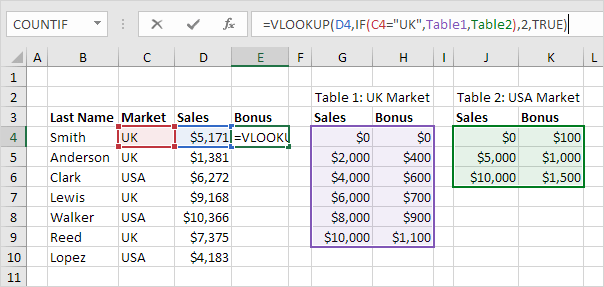
Use VLOOKUP when you need to discover things in a table or a variety by row. For example, search for a rate of a vehicle component by the component number, or discover an employee name based on their staff member ID. In its easiest kind, the VLOOKUP feature states: =VLOOKUP(What you wish to look up, where you intend to seek it, the column number in the variety including the worth to return, return an Approximate or Exact match-- suggested as 1/TRUE, or 0/FALSE).

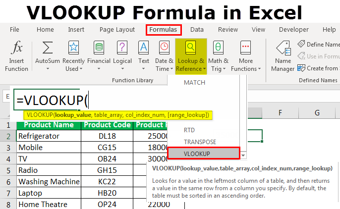
Use the VLOOKUP function to look up a value in a table. Phrase structure VLOOKUP (lookup_value, table_array, col_index_num, [range_lookup] For instance: =VLOOKUP(A 2, A 10: C 20,2, TRUE) =VLOOKUP("Fontana", B 2: E 7,2, FALSE) =VLOOKUP(A 2,'Customer Facts'! A: F,3, FALSE) Disagreement name Description lookup_value (called for) The value you want to seek out. The worth you want to seek out need to be in the first column of the series of cells you specify in the table_array disagreement.

Lookup_value can be a worth or a reference to a cell. table_array (called for) The series of cells in which the VLOOKUP will look for the lookup_value and the return value. You can make use of a named array or a table, and also you can make use of names in the argument instead of cell recommendations.

The cell array also needs to include the return value you intend to locate. Discover just how to choose arrays in a worksheet. col_index_num (needed) The column number (beginning with 1 for the left-most column of table_array) that includes the return worth. range_lookup (optional) A sensible value that specifies whether you want VLOOKUP to discover an approximate or a precise match: Approximate suit - 1/TRUE thinks the first column in the table is arranged either numerically or alphabetically, and will then look for the closest value.

For instance, =VLOOKUP(90, A 1: B 100,2, REAL). Precise match - 0/FALSE look for the exact value in the first column. For example, =VLOOKUP("Smith", A 1: B 100,2, FALSE). There are four items of info that you will certainly require in order to develop the VLOOKUP syntax: The worth you intend to seek out, additionally called the lookup worth.

Some Ideas on How To Use Vlookup You Need To Know

Keep in mind that the lookup worth must constantly be in the very first column in the range for VLOOKUP to function correctly. For example, if your lookup value remains in cell C 2 then your variety must start with C. The column number in the range which contains the return worth. For instance, if you specify B 2:D 11 as the range, you must count B as the initial column, C as the 2nd, and so forth.

If you don't define anything, the default worth will always hold true or approximate match. Now put all of the above together as adheres to: =VLOOKUP(lookup value, array containing the lookup value, the column number in the range containing the return worth, Approximate match (TRUE) or Exact match (FALSE)). Here are a few instances of VLOOKUP: Problem What failed Incorrect worth returned If range_lookup holds true or omitted, the very first column needs to be arranged alphabetically or numerically.

Either kind the very first column, or make use of FALSE for an exact match. #N/ A in cell If range_lookup is TRUE, then if the worth in the lookup_value is smaller sized than the tiniest worth in the first column of the table_array, you'll get the #N/ An error value. If range_lookup is FALSE, the #N/ An error worth shows that the exact number isn't found.

#REF! in cell If col_index_num is above the number of columns in table-array, you'll get the #REF! mistake worth. For even more details on settling #REF! mistakes in VLOOKUP, see Just how to correct a #REF! mistake. #VALUE! in cell If the table_array is less than 1, you'll obtain the #VALUE! error worth.

#NAME? in cell The #NAME? error worth usually implies that the formula is missing out on quotes. To look up an individual's name, see to it you use quotes around the name in the formula. For instance, go into the name as "Fontana" in =VLOOKUP("Fontana", B 2: E 7,2, FALSE). To learn more, see Exactly how to correct a #NAME! error.

The Only Guide to Excel Vlookup

Find out just how to utilize outright cell referrals. Do not keep number or date values as message. When looking number or date worths, be sure the information in the very first column of table_array isn't kept as message worths. Otherwise, VLOOKUP might return an incorrect or unanticipated worth. Sort the very first column Sort the very first column of the table_array before using VLOOKUP when range_lookup is TRUE.

An enigma matches any kind of single personality. An asterisk matches any sequence of personalities. If you wish to discover an actual question mark or asterisk, kind a tilde (~) in front of the character. For example, =VLOOKUP("Fontan?", B 2: E 7,2, FALSE) will search for all instances of Fontana with a last letter that can vary.

When looking message worths in the very first column, make certain the information in the first column doesn't have leading areas, tracking areas, irregular usage of straight (' or") and curly (' or ") quotation marks, or nonprinting personalities. In these cases, VLOOKUP might return an unanticipated value.

You can constantly ask a professional in the Excel Individual Voice. Quick Recommendation Card: VLOOKUP refresher Quick Recommendation Card: VLOOKUP troubleshooting suggestions You Tube: VLOOKUP video clips from Excel neighborhood specialists Every little thing you need to understand about VLOOKUP Just how to deal with a #VALUE! mistake in the VLOOKUP function Exactly how to remedy a #N/ A mistake in the VLOOKUP function Introduction of formulas in Excel Just how to avoid busted formulas Spot mistakes in solutions Excel features (indexed) Excel functions (by classification) VLOOKUP (totally free preview).

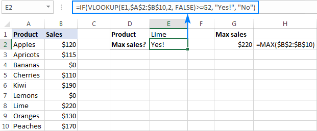
To calculate shipping price based on weight, you can use the VLOOKUP function. In the example shown, the formula in F 8 is: =VLOOKUP(F 7, B 6: C 10,2,1)* F 7 This formula uses the weight to find the correct "price per kg" then ... To override result from VLOOKUP, you can nest VLOOKUP in the IF function.

vlookup excel kutools vlookup excel quick excel vlookup quick reference